Matryoshka Embeddings: Smarter Embeddings with Voyage AI

In the realm of AI, embedding models are the bedrock of advanced applications like retrieval augmented generation (RAG), semantic search, and recommendation systems. These models transform unstructured data (text, images, audio) into high-dimensional numerical vectors, allowing us to perform similarity searches and power intelligent features. However, traditional embedding models often generate fixed-size vectors, leading to trade-offs between performance and computational overhead.

This post will dive deep into Matryoshka Representation Learning (MRL), a novel approach that creates flexible, multi-fidelity embeddings. We’ll compare and contrast MRL with traditional embeddings and quantization, detailing its unique training process and showcasing how Voyage AI’s voyage-3-large and the recently released voyage-3.5 models leverage MRL as well as quantization to deliver unparalleled efficiency with MongoDB Atlas Vector Search.

Understanding embedding models

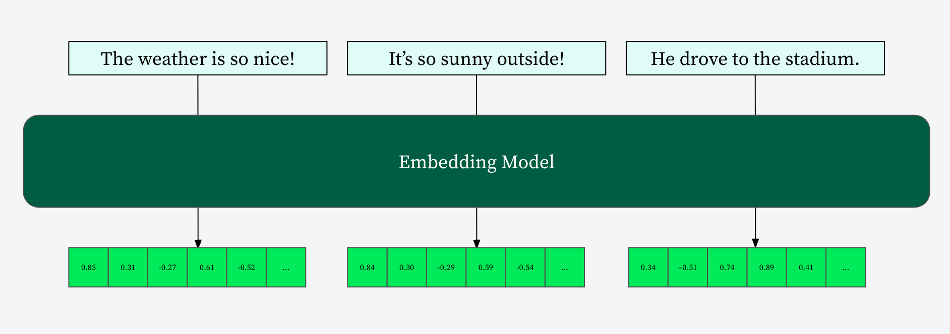
At their core, embedding models learn to represent discrete items (words, sentences, documents) as continuous vectors in a multi-dimensional space. The key principle is that items with similar meanings or characteristics are mapped to points that are close to each other in this vector space. This spatial proximity then allows for efficient similarity comparisons using metrics like cosine similarity.

For example, in a semantic search application, when a user queries “best vegan restaurants,” the embedding model converts this query into a vector. It then compares this vector against a database of pre-computed embeddings for restaurant descriptions. Restaurants whose embeddings are “nearby” the query embedding are deemed relevant and returned to the user.

Figure 1. Example embedding model.

Challenges with traditional embeddings

Historically, embedding models generate vectors of a fixed size, for example, 768, 1024, or 4096 dimensions. While effective, this fixed-size nature presents challenges:

• Inflexibility: A model trained for, say, 768-dimensional embeddings, will suffer a significant performance drop if you simply truncate its vectors to a smaller size, like 256 dimensions, without retraining. This means you’re locked into a specific dimension size, even if a smaller representation would suffice for certain tasks.

• High computational load: Higher-dimensional vectors demand more computational resources for storage, transfer, and similarity calculations. In scenarios with large datasets or real-time inference, this can lead to increased latency and operational costs.

• Information loss on truncation: Without specific training, truncating traditional embeddings inevitably leads to substantial information loss, compromising the quality of downstream tasks.

Matryoshka Representation Learning

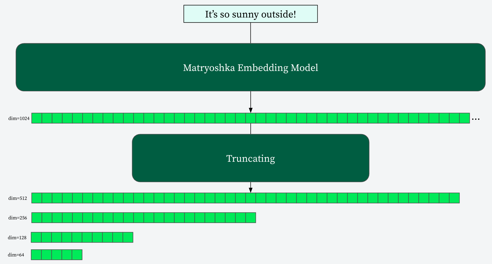
MRL, introduced by researchers from the University of Washington, Google Research, and Harvard University in 2022, offers an elegant solution to these challenges. Inspired by the Russian nesting dolls, MRL trains a single embedding model such that its full-dimensional output can be truncated to various smaller dimensions while still retaining high semantic quality. The magic lies in how the model is trained to ensure that the initial dimensions of the embedding are the most semantically rich, with subsequent dimensions adding progressively finer-grained information.

This means you can train a model to produce, say, a 1024-dimensional embedding. Then, for different use cases or performance requirements, you can simply take the first 256, 512, or any other number of dimensions from that same 1024-dimensional vector. Each truncated vector is still a valid and semantically meaningful representation, just at a different level of detail.

Figure 2. Matryoshka embedding model truncating the output.

Understanding MRL with an analogy

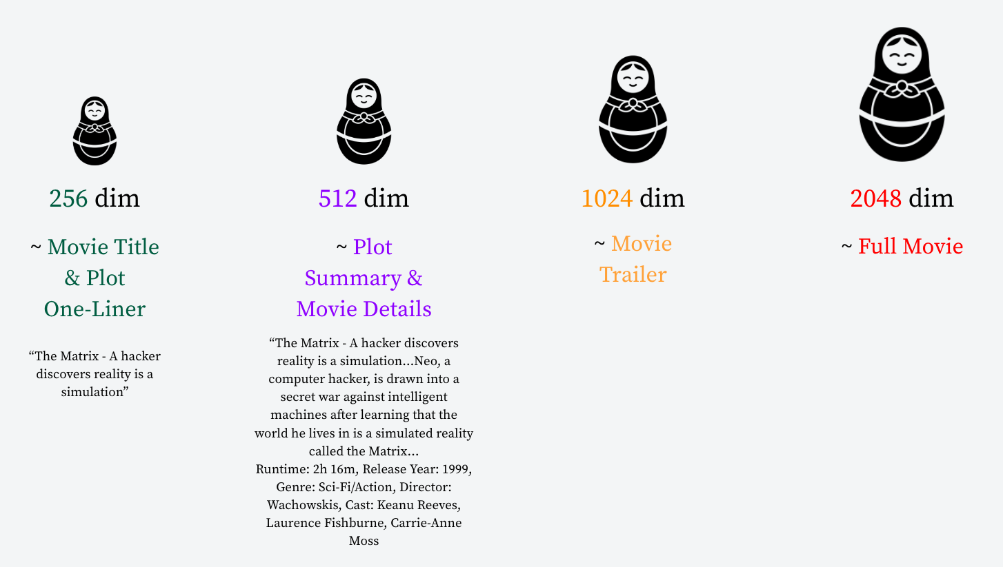
Imagine a movie. A 2048-dimensional MRL embedding might represent the “Full Movie”. Truncating it to:

• 1024 dimensions: Still provides enough information for a “Movie Trailer.”

• 512 dimensions: Gives a “Plot Summary & Movie Details.”

• 256 dimensions: Captures the “Movie Title & Plot One-liner.”

This “coarse-to-fine” property ensures that each prefix of the full vector remains semantically rich and usable. You simply keep the first N dimensions from the full vector to truncate it.

Figure 3. Visualizing the Matryoshka doll analogy for MRL.

The unseen hand: How the loss function shapes embedding quality

To truly grasp what makes MRL distinct, we must first understand the pivotal role of the loss function in the training of any embedding model. This mathematical function is the core mechanism that teaches these sophisticated models to understand and represent meaning.

During a typical training step, an embedding model processes a batch of input data, producing a set of predicted output vectors. The loss function (“J” in the below diagram) then steps in, comparing these predicted embeddings (“y_pred”) against known “ground truth” or expected target values (“y”). It quantifies the discrepancy between what the model predicts and what it should ideally produce, effectively gauging the “error” in its representations. A high loss value signifies a significant deviation – a large “penalty” indicating the model is failing to capture the intended relationships (e.g., placing semantically similar items far apart in the vector space). Conversely, a low loss value indicates accurate capture of these relationships, ensuring that similar concepts (like different images of cats) are mapped close together, while dissimilar ones remain distant.

Figure 4. Training workflow including the loss function.

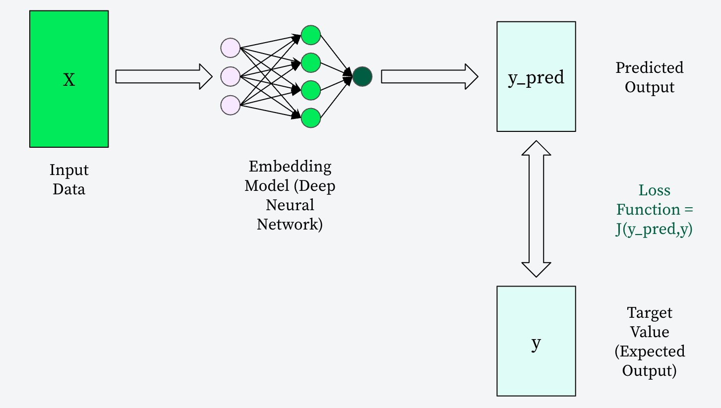
The iterative training process, guided by an optimizer, continuously adjusts the model’s internal weights with the sole aim of minimizing this loss value. This relentless pursuit of a lower loss is precisely how an embedding model learns to generate high-quality, semantically meaningful vectors.

MRL training process

The key differentiator for MRL lies in its training methodology. Unlike traditional embeddings, where a single loss value is computed for the full vector, MRL training involves:

1. Multiple loss values: Separate loss values are computed for multiple truncated prefixes of the vector (e.g., at 256, 512, 1024, and 2048 dimensions).

2. Loss averaging: These individual losses are averaged (or summed), to calculate a total loss.

3. Incentivized information packing: The model is trained to minimize this total loss. This process penalizes even the smallest prefixes if their loss is high, strongly incentivizing the model to pack the most crucial information into the earliest dimensions of the vector.

This results in a model where information is “front-loaded” into early dimensions, ensuring accuracy remains strong even with fewer dimensions, unlike traditional models where accuracy drops significantly upon truncation. Examples of MRL-trained models include voyage-3-large and voyage-3.5.

MRL vs. quantization

It’s important to differentiate MRL from quantization, another common technique for reducing embedding size. While both aim to make embeddings more efficient, their approaches and benefits differ fundamentally.

Quantization techniques compress existing high-dimensional embeddings into a more compact form, by reducing the precision of the numerical values (e.g., from float32 to int8). The following table describes the precise differences between MRL and Quantization.

Aspect	MRL	Quantization
Goal	Reduce embedding dimensionality (e.g., 256 out of 2048 dims)	Reduce embedding precision (e.g., instead of using fp32, using int8/binary embeddings)
Output Type	Float32 vectors of varying lengths	Fixed-length vectors with lower bit representations
Training Awareness	Uses multi-loss training across dimensions	Often uses quantization-aware training (QAT)
Use Case	Trade-off accuracy vs compute/memory at inference	Minimize storage and accelerate vector math operations
Example (Voyage AI)	voyage-3-large @ 512-dim-fp32	voyage-3-large @ 2048-dim-int8

Flexibility and efficiency with MRL

The core benefit of MRL is its unparalleled flexibility and efficiency. Instead of being locked into a single, large vector size, you can:

• Choose what you need: Generate a full 2048-dimensional vector and then slice it to 256, 512, or 1024 dimensions based on your specific needs.

• One vector, multiple fidelities: A single embedding provides multiple levels of detail and accuracy.

• Lower compute, bandwidth, and storage: By using smaller vector dimensions, you drastically reduce the computational load for indexing, query processing, and data transfer, as well as the storage footprint in your database.

• Efficient computation: The embedding is computed once, and then you simply slice it to the desired dimensions, making it highly efficient.

Voyage AI, in particular, leverages MRL by default across its models, including voyage-3-large and the latest voyage-3.5, enabling scalable embeddings with one model and multiple dimensions. This allows you to dynamically choose between space/latency and quality at query time, leading to efficient retrieval with minimal accuracy loss.

Voyage AI’s dual approach: MRL and quantization for ultimate efficiency

Voyage AI models maximize efficiency by combining MRL and quantization. MRL enables flexible embeddings by allowing you to select the optimal vector length—for instance, using 512 instead of 2048 dimensions—resulting in significant reductions in size and computational overhead with minimal accuracy loss. Quantization further compresses these vectors by reducing their bit precision, which cuts storage needs and speeds up similarity search operations.

This synergy allows you to choose embeddings tailored to your application’s requirements: a voyage-3-large embedding can be used as a compact 512-dimensional floating-point vector (leveraging MRL) or as a full 2048-dimensional 8-bit integer vector (via quantization). The dual approach empowers you to balance accuracy, storage, and performance, ensuring highly efficient, flexible embeddings for your workload. As a result, Voyage AI models deliver faster inferences and help reduce infrastructure costs when powering applications with MongoDB Atlas Vector Search.

This article first appeared on Read More