Discover Rich, Graph-Powered Insights in Your BigQuery Data

Businesses increasingly win and lose based on how effectively they extract insight from their data. There are several ways to get more value from existing infrastructure: you can collect more data, build more complex models, or reorganize the data you already have to uncover patterns that weren’t visible before. That last approach is where graph modeling and graph algorithms come in, revealing influence, centrality, communities, and hidden relationships across connected data. 

Importantly, you don’t need to set up separate infrastructure outside of BigQuery to generate these richer insights. As datasets grow, traditional open-source tools like NetworkX can struggle to scale beyond a single machine, but Aura Graph Analytics delivers scalable graph processing with minimal operational overhead. In the below example, you’ll see how Aura Graph Analytics fits naturally into a BigQuery workflow: query your data, load it into a Pandas DataFrame, run powerful graph algorithms directly in Python, and—if desired—write enriched results back to the warehouse, all within a familiar, pay-as-you-go environment that separates compute from storage.

Graph Analytics + BigQuery

Neo4j built Aura Graph Analytics to work with enterprise data wherever it lives — including BigQuery. Connecting to your BigQuery data is straightforward. Here’s the flow.

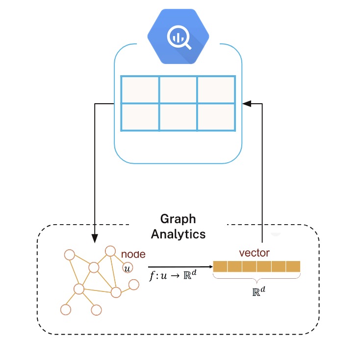
First, write a SQL query in BigQuery to extract the data you want to model as a graph, and load the results into Python dataframes. Typically, you’ll create one dataframe for nodes and another for relationships (an edge list).

Next, start a session on Aura’s serverless infrastructure and project the graph into memory. A graph projection is an in-memory representation optimized specifically for running graph algorithms.

Once projected, you can run algorithms on Aura’s compute. In the diagram shown on the left, we use an embedding algorithm to generate vector representations of nodes, which are then written back into a Python dataframe.

From there, you can use these graph-derived features in downstream machine learning workflows — or write them back to BigQuery for broader analytics and operational use.

Getting Our Data

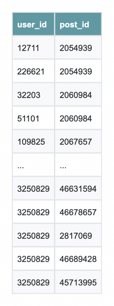
We’ll use data from one of BigQuery’s public datasets to create a manageable subgraph of Stack Overflow comments.

The query begins by selecting a highly active post with many distinct commenters to act as a hub. It then gathers all comments on that hub (the first hop) and expands outward to capture other posts commented on by those same users (the second hop). Finally, it includes all comments on those second-hop posts.

This approach yields a compact, mostly connected user–post subgraph that’s ideal for running graph algorithms like WCC or PageRank in a demo, while keeping the data volume small and easy to work with.

%%bigquery df
WITH hub_post AS (
  SELECT post_id
  FROM `bigquery-public-data.stackoverflow.comments`
  WHERE user_id IS NOT NULL
  GROUP BY post_id
  ORDER BY COUNT(DISTINCT user_id) DESC
  LIMIT 1
),

-- 2) First hop: all comments on the hub post
h1_comments AS (
  SELECT user_id, post_id
  FROM `bigquery-public-data.stackoverflow.comments`
  WHERE post_id IN (SELECT post_id FROM hub_post)
    AND user_id IS NOT NULL
),

-- 3) Second hop: all other posts commented on by those users
h2_posts AS (
  SELECT DISTINCT c.post_id
  FROM `bigquery-public-data.stackoverflow.comments` c
  JOIN h1_comments h1
    ON c.user_id = h1.user_id
  WHERE c.post_id != h1.post_id
),

-- 4) Bring in all comments on those second-hop posts
h2_comments AS (
  SELECT user_id, post_id
  FROM `bigquery-public-data.stackoverflow.comments`
  WHERE post_id IN (SELECT post_id FROM h2_posts)
    AND user_id IS NOT NULL
)

-- 5) Final connected slice: hub post + second-hop posts
SELECT user_id, post_id
FROM h1_comments
UNION ALL
SELECT user_id, post_id
FROM h2_comments

The results are saved as df and are nearly ready for use with Neo4j Aura Graph Analytics.

Setting Up Graph Analytics

First, we download the package:

!pip install graphdatascience

Then we import all the necessary packages

from graphdatascience.session import DbmsConnectionInfo, AlgorithmCategory, CloudLocation, GdsSessions, AuraAPICredentials
from datetime import timedelta
import pandas as pd
import os
from google.colab import userdata

Then we create a session using our Aura credentials. Please note that you will need an Aura account with Graph Analytics to follow along:

CLIENT_ID = 'your_client_id'
CLIENT_SECRET = 'your_client_secret'
TENANT_ID = 'your_tenent_id'

from graphdatascience.session import GdsSessions, AuraAPICredentials, AlgorithmCategory, CloudLocation
from datetime import timedelta

sessions = GdsSessions(api_credentials=AuraAPICredentials(CLIENT_ID, CLIENT_SECRET, TENANT_ID))

name = "my-new-session-sm"
memory = sessions.estimate(
    node_count=20,
    relationship_count=50,
    algorithm_categories=[AlgorithmCategory.CENTRALITY, AlgorithmCategory.NODE_EMBEDDING],
)
cloud_location = CloudLocation(provider="gcp", region="europe-west1")

gds = sessions.get_or_create(
    session_name=name,
    memory=memory,
    ttl=timedelta(hours=5),
    cloud_location=cloud_location,
)

Then we do some data cleaning to get it into the right format:

# Drop any rows with negative IDs
df = df[(df["user_id"] >= 0) & (df["post_id"] >= 0)]

# Nodes
users = pd.DataFrame({
    "nodeId": df["user_id"].dropna().unique(),
})
users["labels"] = [["User"]] * len(users)

posts = pd.DataFrame({
    "nodeId": df["post_id"].dropna().unique(),
})
posts["labels"] = [["Post"]] * len(posts)

nodes = pd.concat([users, posts], ignore_index=True)

# Relationships (bipartite edges: User -> Post, and reverse for undirected WCC)
rels_forward = pd.DataFrame({
    "sourceNodeId": df["user_id"],
    "targetNodeId": df["post_id"],
    "relationshipType": "COMMENTED_ON"
})
rels_reverse = pd.DataFrame({
    "sourceNodeId": df["post_id"],
    "targetNodeId": df["user_id"],
    "relationshipType": "COMMENTED_ON"
})

relationships = pd.concat([rels_forward, rels_reverse], ignore_index=True).drop_duplicates()

Creating our Graph and Running Algorithms

Next, we create a graph projection using the gds.graph.construct method. This will create an in-memory graph to run algorithms against

if gds.graph.exists("so_comments_bip")["exists"]:
    gds.graph.drop("so_comments_bip")
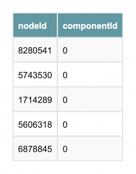
G = gds.graph.construct("so_comments_bip", nodes, relationships)

First, we will check that all of our components are in the same community using Weakly Connected Components. If this is true, then we can reach any given node from any other node; that is, the graph is connected.

wcc = gds.wcc.stream(G)   # returns a pandas DataFrame with columns: nodeId, componentId, size (version-dependent)

Because they all have the same componenetId we can deduce that they in fact are in the same community, and thus, the whole graph is connected. And with that simple Python call, we can perform a tedious data validation task that would otherwise be tedious. 

Next, we run PageRank on the connected subgraph to identify the most influential nodes.

PageRank doesn’t just count connections—it weighs the quality of those connections, highlighting users or posts that sit at the center of discussion. By looking at the top results, we can quickly see which nodes are structurally important in the network and would be the most impactful to investigate further.

And as a fun bonus trivia bit, PageRank was originally developed to power Google!

# Run PageRank (stream results back to Pandas)
pr = gds.pageRank.stream(
    G,
    maxIterations=20,
    dampingFactor=0.85
)

# Sort and inspect the top results
pr_sorted = pr.sort_values("score", ascending=False)
pr_sorted.head(10)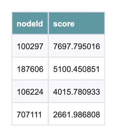

From here, the enriched DataFrame can be written back to your database or used directly in downstream machine learning workflows for tasks like feature engineering, ranking, or anomaly detection. What you’ve seen here is just one example — explore the full suite of graph algorithms to uncover communities, detect similarity, compute influence, and generate embeddings that unlock even deeper insight from your connected data.

This article first appeared on Read More